Numerical Parallel Algorithms

Systems of Linear Equations

• Find x₀, x₁, ..., x_n-1 such that
  a_0,0 x₀ + a_0,1 x₁ + ... + a_0,n-1 x_n-1 = b₀
  a_1,0 x₀ + a_1,1 x₁ + ... + a_1,n-1 x_n-1 = b₁
  ...
  a_n-1,0 x₀ + a_n-1,1 x₁ + ... + a_n-1,n-1 x_n-1 = b_n-1
  
  
• In matrix form we can write Ax = b, where A is an n x n matrix, and x and b are vectors of size n.
• Numerous applications.

Gauss Elimination

• A commonly used method to solve systems of linear equations. A x = b,
• The objective is to turn the matrix A into a triangular one.
• We start by multiplying the first row by a constant then subtracting it from the second one such that the first element in the second row becomes 0.
• We repeat this for each remaining row.
• A triangular system of linear equations is easy to solve.
• Time complexity: O(n³).

Sequential Algorithm

for (i=0; i < n-1; i++) { 
   for (j=i+1; j < n; j++) { 
      m = a[j][i]/a[i][i]; // multiplier
      for (k=j; k < n; k++){ 
         a[j][k] = a[j][k] - a[i][k]*m;
      }
      b[j]=b[j] - b[i]*m; // adjust b too
   }
}

Computing the Solution

x[n-1] = b[n-1]/a[n-1][n-1]; 
for (i=n-2; i >= 0; i--) { 
   r = b[i];
   for (j=i+1; j < n; j++) 
      r = r - a[i][j]*x[j]; 
   x[i] = r / a[i][i];
}

Gauss Elimination

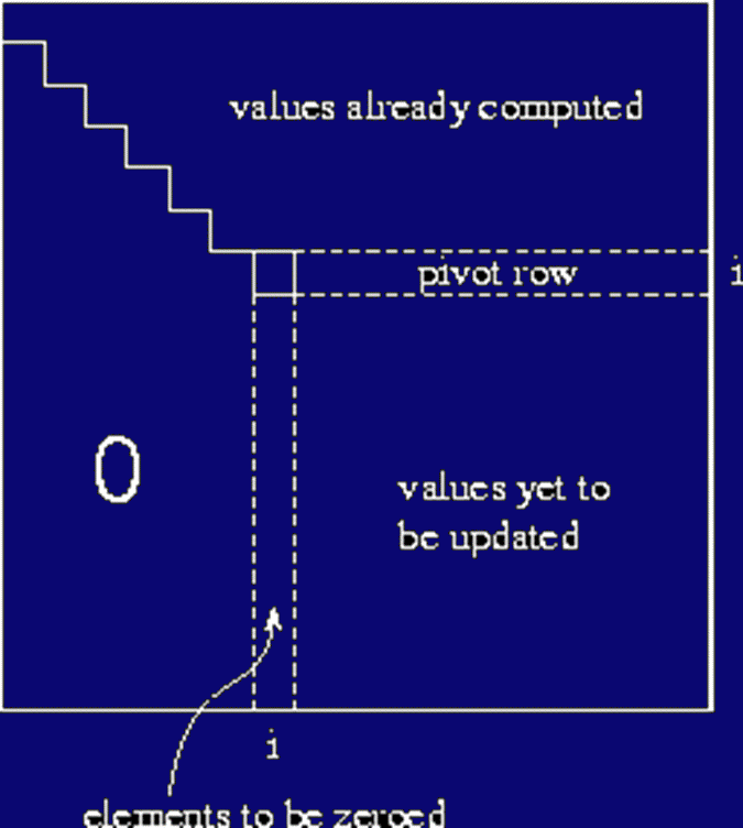
• In step i the first non-0 element of the row i is a_i,i. The corresponding element in row j is a_j,i. To eliminate this element, we need to multiply row i by -a_j,i/a_i,i and add it to row j.
• All the other elements on row j are computed as
  a_j,k = a_j,k - a_k,i *a_j,i/a_i,i
• Partial pivoting: if a_i,i is small, this could lead to numerical errors. One can swap row i with the row containing the largest value in column i and use it as pivot.

Parallel Implementation

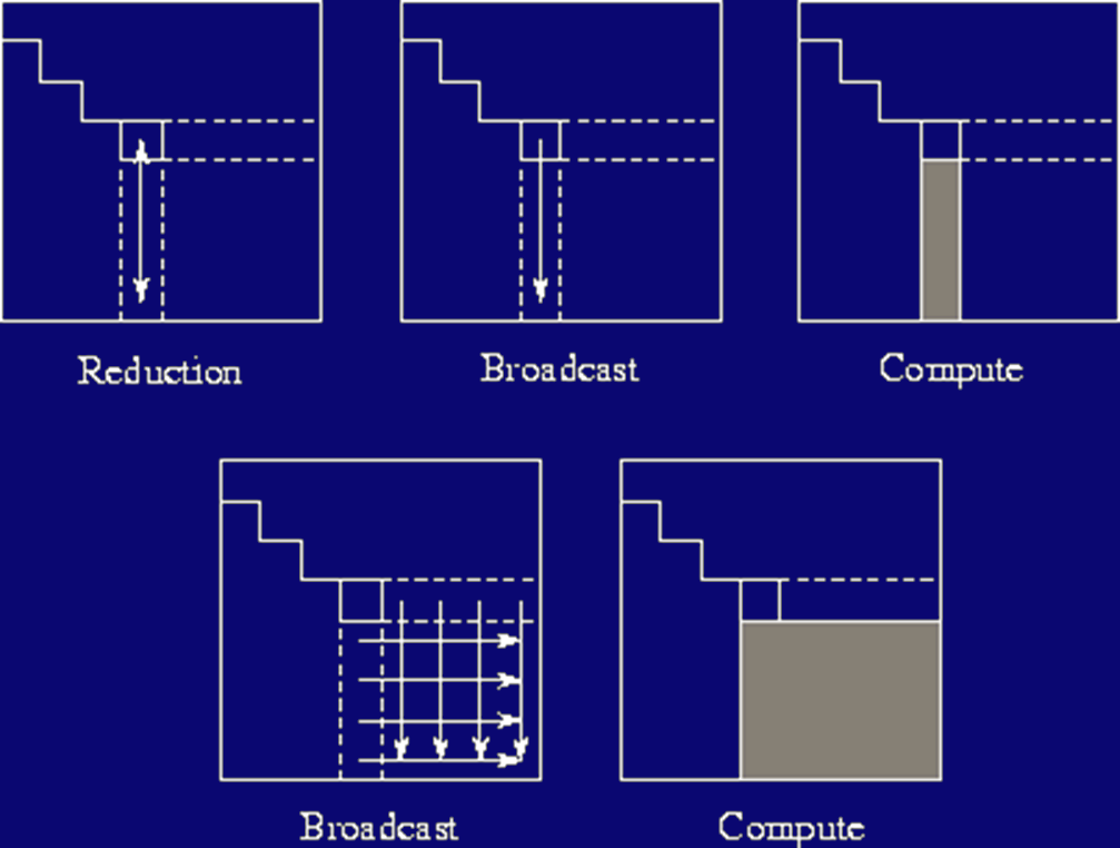
• Division by rows. For every row i to be eliminated, each process can compute a row j.
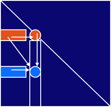
• For every element a_j,k to be computed by P_j, the process will need the element a_i,k. It's the same element for each process.
• The master in each step would be P_i. It would have to broadcast a[i][k] for k from i to n-1.
• The processes would have to do the computations in synch.
• Complexity: O(n²) with O(n²) communication.

Parallel idea:

Improvements

• Broadcast the whole row in each iteration to reduce some of the overhead.
• Each process stops computing after the elimination finishes its row.
• If we use less than n processes, then we can assign them one row at a time then start over. Process 0 would handle rows 0, np, 2*np, .... Process 1 would handle rows 1, np+1, 2*np+1, etc.
• This is called a cyclic stripped partitioning and it balances the load better.

Jacobi Iteration

• Computing a solution by repeatedly getting closer to it.
• Start from some random values for x. Then compute
  x^k+1_i = (1/a_i,i)(b_i - Sum _{j != i} a_i,j x^k-1_j)
• We repeat the procedure until the difference becomes insignificant.
• It can be shown that xk with this procedure will converge towards the solution of the system.

Parallel Version

• Each process can compute one value in x. With n processes, the complexity of one iteration is n.
• For certain classes of matrices (such as, diagonally dominant) the algorithm will converge to a "good" solution in O(log(n)).

Cholesky Decomposition

• Given a symmetric positive definite matrix A, the Cholesky decomposition is a lower triangular matrix L such that A = L L^T.
• A matrix A is called positive definite if x^T A x > 0 for every nonzero vector x.
• L is also called computing the square root of the matrix A.
• One of the fastest decompositions available, a special case of the LU decomposition.

Method

• We start by computing for every column
  L_ii = sqrt(a_ii - Sum_k=1^i-1 L_ik²)
  
  
• Then the rest of the elements:
  L_ji = (1/L_ii) (a_ij - Sum_k=1^i-1 L_ikL_jk)
  
  
• We notice that in the previous formula, computing an element depends on the diagonal element on the same column and on elements before it on the same line.
• The best way to compute this is having the threads advance in the matrix parallel to the second diagonal.

Compute a Cell of L

float Compute_cell(i, j) {
   x = a[i, j];
   for (k=0; k < i && k < j; k++)
      x -= a[i,k]*a[j,k];
   if (i != j)
      x = x/a[i,i];
   else
      x = sqrt(x);
   return x;
}

Sequential Algorithm

Cholesky() {
   for (i=0; i < n; i++)
      for (j=i; j < n; j++)
         a[i,j] = Compute_cell(i, j);
} 

Workers

• Advancing on lines parallel to the second diagonal.
• Definition of such a line:
  row + col = d
  where d is constant for each line and goes from 0 to 2*(n-1).

Parallel Algorithm

Cholesy_Worker(thread_no) {
   col = id;
   for (d=0; d < 2*n-1; d++) {
      if (d >= 2*col && d < n + col) {
         row = d – col;
         a[row,col] = Compute_cell(row, col);
      }
      Barrier(thread_no);
   }
}

LU Decomposition

• Successive elimination of variables can be used to solve the linear system Ax = b, method called Gaussian elimination.
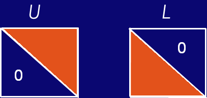
• The LU decomposition factors the matrix A as a product of upper and lower triangular matrices (U and L, respectively).
  A_ij = Sum_k=1^min(i,j) L_ik U_kj
• Then the system can be solved the following way:
• Solve Ly = b, where y is a vector,
• Solve Ux = y, where x is the solution to the initial equation.

Sequential Algorithm

• The elements on the diagonal of L can be chosen to be 1. This way we can store both L and U in the matrix A itself.
• We don't need the previous rows in the computation. L[i,i] = 1.

Sequential Algorithm

for (j = 1; j < n; j++)
   for (i = 1; i < j; i++) {
      U[i][j] = A[i][j];
      for (k = 1; k < i; k++) 
         U[i][j] -= L[i][k] * U[k][j];
   }
   for (i = j+1; i < n; i++) {
      L[i][j] = A[i][j];
      for (k = 1; k < j; k++) 
         L[i][j] -= L[i][k] * U[k][j];
      L[i][j] /= U[j][j];
   }
}

Parallel Version

• Usual decomposition: blocks of rows. Load balancing problems can occur.
• Typical problem used for benchmarking and demos.
• Partial pivoting also used here: find the row with the largest pivot and substitute the first one with it.
• Particularly efficient versions exist for sparse matrices.
• A demo of PLapack

Linear Algebra Libraries

• Known ones in C/C++:
• LAPACK - linear algebra package
• ScaLAPACK - Scalable Linear Algebra Package
• PLAPACK - parallel Lapack, MPI-based
• PLASMA - Parallel Linear Algebra for Scalable Multi-core Architectures
• MAGMA - Matrix Algebra on GPU and Multicore Architectures