Machine Learning

Outline

• Introduction
• Learning from observations
• Statistical learning
• Reinforcement learning
• Specialized algorithms:
• neural networks
• genetic/evolutionary algorithms
• SOM

Machine Learning

• Machine Learning is the study of computer algorithms that improve automatically through experience.
• "Find a bug in a program, and fix it, and the program will work today. Show the program how to find and fix a bug, and the program will work forever."
  - Oliver G. Selfridge, in AI's Greatest Trends and Controversies
• "Given a task we want the computer to do, the idea is to repeatedly demonstrate how the task is performed, and let the computer learn by example, i.e., generalise some rules about the task and turn these into a program." - Simon Colton

Motivation

• Some problems can be hard to solve by hand and an ML system can be a more robust approach.
• Adaptable problems: we can't predict beforehand all the situations that the agent will have to deal with.
• Customizing: a program that adapts to specific interests of users.
• Data mining: a better understanding of large amounts of data, inferring knowledge from it.

Problem Examples

• Hard to solve: playing chess, driving an airplane, predicting the weather.
• Adaptable: sending an autonomous vehicle to an unexplored planet.
• Customizable: learning client preferences, predicting market strategies, recognizing someone's handwriting, carrying a friendly and knowledgeable conversation.
• Data mining: finding the correlation between various factors and hard to cure diseases.

Issues in ML

• Choosing the model that can best approximate the function we're looking for.
• Number of training examples and accuracy.
• Dealing with noisy data.
• Are there limits to what the algorithm can learn?
• How can prior experience be used?
• Complexity of hypothesis/ changes in the representation.
• Examples from biological systems.

Types of Learning

• Supervised learning - the algorithm must build a model (a function) that maps a set of input values to some known output.
• Unsupervised learning - it must find a model to fit the observations without knowing the output a priori.
• Reinforcement learning - learning from examples based on positive/negative feedback.
• Transduction - learning a model from a set of data with hope to apply it to a new set of data.

Training Set - Testing Set

• The algorithm is given a set of data with known output - this is the training set.
• Once a model is derived, it must be applied to a new set of objects - test set.
• The performance of the system on the training set is called retrospective evaluation. The performance on the test set is considered the real one.
• Example: we want to learn the moving patterns of clouds in a given area. Training set: collect data on the clouds over 2 years. Test set: new data for the next year.

Crossvalidation

• Suppose we have a set T of N data samples with known output. We want to divide it into a train set and a test set optimizing the use of the data.
• We divide the N samples into K sets of equal size, T₁, T₂, ... T_k.
• We perform K experiments. For each i,
• 1 < i < K, the training set is T/T_i and the test set is T_i.
• The performance of the model is evaluated as the average over the K individual results from these experiments.

Learning from Observations

• Suppose a learning agent contains a performance component that makes decisions about actions to be taken.
• What parts of the performance component should be learned?
• What feedback is available for the agent to learn from?
• What representation we use to allow for the learning process to take place and to store the acquired knowledge for later use?
• Learning a continuous function is called regression. Learning a discrete one is called classification.

Inductive Learning

• Problem: finding a general expression for a function f given some examples.
• Example: a pair (x, f (x)).
• The program will return a function h that approximates f. h is called a hypothesis.
• Induction problem: how general is the solution h and how well does it predict unseen examples. Also known as extrapolation.
• Consistent hypothesis: h is called consistent if it agrees with all the data, meaning h(x) = f(x) for all the provided examples.

Consistency Problem

• Continuous functions: they can usually be approximated by polynomials of degree at least equal to the number of examples -1.
• Ockham's razor: if several consistent hypothesis are available for the same function f, choose the simplest one.
• Hypothesis space H: defined by the shape chosen for the function. We say that the problem is realizable if the function f belongs to the hypothesis space.

Learning Decision Trees

• Decision tree - component of an expert system. They can be seen as a classification system.
• Suppose we have a training set consisting of {(x1, y1), (x2, y2), ..., (xn, yn)} where y1, y2, ..., yn represent k different classes.
• General algorithm: find the best attribute that separate the most of the input values in classes.
• For each group resulting from the first operation, if the separation is not perfect, find a second attribute that best distinguishes between the classes.
• Repeat until the tree is consistent.

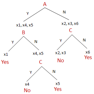
Example - Boolean Tree

A B C Answer x1 Y Y Y Yes x2 N N Y No x3 N N Y No x4 Y N Y No x5 Y N N Yes x6 N Y N Yes

Overfitting

• Overfitting: training some flexible representation so that it memorizes the data but fails to predict well in the future.
• The algorithm finds "patterns" or "regularities" in the data that fit the training set but are contradicted by the test set.
• Avoiding it:
• have a large enough sample set.
• Make sure there are no patterns in the way the sample points are chosen.
• Interpolate between several predictors.

Ensemble Learning - Boosting

• Given a set of predictors, P₁, P₂, ..., P_m for a set of classes C₁, C₂, ..., C_k.
• For each of them, we can learn the probability that a particular prediction is correct from the data. w_ij = P(class(x)=C_j | P_i(x) = C_j)
• This translates into a set of weights associated with each class for each predictor.
• To classify an object, we apply each predictor to obtain a class. The result is a weighted sum of the predictions:
• C(x) = S_i w_ij P_i(x) where P_i(x) = C_j.

Parametric Learning

• Parametric learning: where the program is learning a hypothesis that has a specific mathematical formula where the things to be learned are some parameters involved in it.
• Non-parametric learning: where the hypothesis can grow with the data, or where it's not expressed in terms of parameters.
• Also called instance-based, or case-based, or memory-based learning. It constructs the hypothesis directly from the training examples.

PL - Example

• Suppose we want to learn the behavior of a population, like the number of hours they watch TV every day.
• We'll assume that this follows a Gaussian distribution with the equation:
  
• Where sigma is the average over the population and mu is the standard deviation.
• We can compute these two parameters (sigma, mu) from the training set.

Nearest Neighbors

• Non-parametric learning. Given a training set of examples and a new object, the algorithm must return the class of the object.
• Somewhat similar to the ensemble learning, but for the case where we can define some distance between the objects to classify.
• It assumes that the properties of a particular object are similar to those objects close to it.
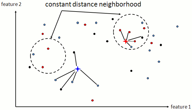
• For each object, we select a neighborhood (a set of objects close to it) and report a classification of the object as the most frequent class in this neighborhood.

k-Nearest Neighbors

• Selecting a neighborhood:
• If the neighborhood is too small, we might not have enough evidence to classify the object.
• If the neighborhood is too large, the significance of the evidence will be diluted.
• To ensure a uniform number of sample points for decision, the neighborhood is defined as the set of k samples that are the closest to the object to classify.
• Eventually the neighbors can be weighted by the distance to the object (their importance in the decision).

5-Nearest Neighbors

Distance

• To apply this method we need a good distance metric.
• The Euclidian distance is ok when the dimensions are well balanced. Otherwise we can use the normalized Euclidian distance:
  
• If the features have discrete values, we can use the Hamming distance: the number of features that are different for two objects.

Kernel Models

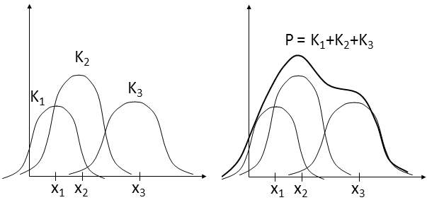
• Each of the training samples xi generates a density function or kernel around it K(x, xi) that peaks at the point xi itself and decreases (normally) as we go away from it.
• The estimation function is a sum of all of these kernel functions:
• P(x) = 1/n S_i=1,n K(x, x_i)
• where K(x, x_i) could be the Gaussian distribution where (x-m) is substituted by the distance D(x, x_i).

Reinforcement Learning

• Learning from success and failure, from rewards and punishments.
• The agent receives some feedback on the result of each action, and it is negative or positive.
• This is related to the utility function (search algorithms). The difference is that the agent doesn't know the utility beforehand. It can only find it out by perception after the action is performed.
• The agent must find an action policy that maximizes the feedback in the long run.

Feedback

• Internal versus external: being hungry and in poor health can be seen as negative feedback.
• A game of tennis: getting the ball in a correct place in the opposite side of the terrain is positive; scoring a point is better; losing a point is negative.
• Trying to pick up a target object with a robot arm: getting close to the object, positive; grasping the object, better; crushing the object, negative, dropping the object, negative.
• The feedback is usually quantifiable. A stronger positive feedback will influence the learning more.

Types of RL

• Utility-based learning - learns a utility function for actions from any given state.
• Q-learning - learns an action-value function that associates a value with each action (does not need states and representation of the environment).
• Reflex agent - learns a direct mapping from states to actions.
• Passive learning - the policy is fixed, the agent must learn the utility function.
• Active learning - the agent must learn the policy (what to do).

Typical Problem Description

• Given the following:
• a set of states S
• a set of actions A
• a set of rewards R :S->R
• the agent must learn a policy p :S->A that maximizes the reward over a sequence of states (s₁, s₂, ..., s_n), defined as
• R_n = R(s₁)+R(s₂)+...+R(s_n).
• The sequence of states is defined as a Markov chain defined by the actions taken by the policy:
• if a_i = p(s_i), then s_i+1 = a_i (s_i)

Example - Riding a Bike

• States: (angle, speed, handlebar).
• Goal: to advance and not to fall.
• Positive feedback: if it went forward and it didn't fall.
• Negative feedback: falling down, being stationary.
• Actions: lean left/right, pedal, turn the handlebar.
• Learning: a set of rules, like
• if angle > 40 and speed < 20, then don't lean more.
• if speed > 5 then don't put your foot down.
• if speed > 5 then increase pedaling.

k-Armed Bandit

• Suppose you have k gambling machines (known as one-armed bandit). Each of them has a probability p_i of winning (0/1), unknown.
• The player has n pulls total. The goal is to maximize the profit.
• One has to try and do both: estimate the probability of winning from each machine, and playing the optimal ones to win the most points.
• This is known as the exploration versus exploitation problem: how many of your pulls you use to learn the probabilities, and how many to actually play?