Local Search
C463 / B551 Artificial Intelligence
Local Search
Local Search
- They apply mostly to problems for which we don't need to know the path to the solution but only the solution itself.
- They operate using a single state or a small number of states and explore the neighbors of that state. They usually don't store the path.
- A particular case are optimization problems for which we search for the best solution according to an objective function.
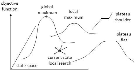
- The distribution of values of the objective function in the state space is called a landscape.
State Space Landscape
- Global maximum - a state that maximizes the objective function over the entire landscape.
- Local maximum - a state that maximizes the objective function in a small area around it.
- Plateau - a state such that the objective function is constant in an area around it.
- Shoulder - a plateau that has an uphill edge.
- Flat - plateau whose edges go downhill.
- Ridge - sequences of local maxima.
- See Fig. 4.10 (pg 111) & 4.13 (pg 114) from the textbook.
Landscape

Hill Climbing
- From the current state it moves to adjacent states going uphill.
- The algorithm ends when it reaches a peak (local or global maximum).
- Simplest version: greedy local search. Expand the current state and move on to the best neighbor.
- Sideways move: when reaching a plateau, jump somewhere else and restart the search. There might be a
limit to the number of sideway moves allowed.
Variations of Hill Climbing
- Stochastic HC: chose randomly among the neighbors going uphill.
- First-choice HC: generate random successors until one is better. Good for states with high numbers of neighbors.
- Random restart: the sideway moves restart from a random state.
- Evolutionary hill-climbing: represents potential solutions as strings and performs random mutations.
Keeps the mutations that are better states. It's a particular case of first-choice and the ancestor of the genetic algorithms.
Continuous Spaces
- When the objective function is continuous. Then the graph of the function creates a
continuous subspace (like a surface) of the landscape.
- Gradient search: if the function is a scalar field of 3 variables, f(x, y, z) in R3, then the gradient of this function:

- gives us the direction where the scalar field grows the most.
- The search moves from s=(x, y, z) to
 .
.
- A plateau is defined by
 .
.
Simulated Annealing
- Random walk: move from the current state to a random neighbor.
- Simulated annealing: combining hill climbing with random walk.
- Annealing: the process of bringing liquid metal down from a high temperature to crystallize into the desired structure.
- We start from a high energy state and we try to reach a low energy state (low cost). It's a minimizing instead of maximizing algorithm.
- Start with a random initial state of energy E and temperature T. Perturb the state randomly to obtain a neighbor. Let DE be the change in energy between the states.
- The energy is a measure of how disturbed a state is from the optimal solution.
The temperature starts high and it slowly goes down with time. This means that "bad moves" are
allowed more easily at the beginning than later on.
- If DE<0, move to the neighbor. This means that the neighbor is a state of lower energy. This part is hill-climbing.
- If DE>0, move to the neighbor with a probability depending on the Boltzmann factor: e-DE/T.
Example: 8-Tile Puzzle
- Place: where each tile I should go. Place(i)=i.
- Position: where it is at any moment.
- Energy: sum(distance(i, position(i))), for i=1,8.
- Energy(solution) = 0
- Random neighbor: from each state there are at most 4 possible moves. Choose one randomly.
- T = temperature. For example, we start with T=50, and at every iteration we decrease it by 1. If T=1 then we stop decreasing it.
Initial state : 
Energy = (2-1)+(6-2)+(7-3)+(4-1)+(8-5) +(6-4)+(7-3)+(9-8) = 1 + 4 + 4 + 3 + 3 + 2 + 4 + 1 = 22
Neighbors: 
Suppose T = 40. Then the probability of the first neighbor is e-(25-22)/40 = 0.9277 = 92.77%
Genetic Algorithms
- The potential solutions are represented as strings over a base alphabet (0/1). The strings are called chromosomes or individuals and their elements are called genes.
- Each chromosome is evaluated by a fitness function.
- The search starts with a number of random chromosomes called initial population.
- From each set of chromosomes called generation we build a new one applying selection, crossover, and mutation. The first generation is the initial population.
- The search continues until a given value for the fitness is achieved or for a given number of generations.
Genetic Operators
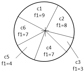
- Fitness-proportionate selection: chooses a chromosome from the population giving a higher probability to those of higher fitness value.
- Crossover: starts with 2 chromosomes (parents), chooses a random position, and swaps the parents' genes to the right of that position. It results in two new chromosomes called children or offspring.
- Mutation: choosing a random gene in an individual and replacing it by another possible random value (1->0, 0->1).
Crossover:
CAA | GTTTAAG
GCT | AAGGTAC
-------------
CAA | AAGGTAC
GCT | GTTTAAG
Mutation:
001110110001 -> 001010110001
Fitness-proportionate selection:
